
Introduction
This past year has been informational, learning from operationalizing machine learning models, this post is an introduction to Machine learning operations henceforth referred to as MLOPs. The term MLOPs in this essay simply refers to the set of practices that deal with the deployment and maintenance of ML model production pipelines reliably. A pipeline is simply the series of steps that are taken to produce a model from data. The goal of MLOPs is operationalizing the series of steps in the processes of creating, serving, deploying, and finally updating the model. The pipeline makes the steps repeatable and reliable
The process of reliably deploying machine learning model pipelines in production is hard. The first challenge is that machine learning unlike software engineering needs existing data for the problem and sourcing data is hard. Machine learning data comes in many forms, however, the four primary data types are numerical data, categorical data, time series data, and text data.
Numerical data is simply quantifiably measured data. Things like age, weight, etc. Exact or whole numbers are discrete numbers, and numbers occurring within a range like a temperature of 27.7F are continuous numbers. Categorical data are attributes defining data e.g ethnicity, and religion. This data is important in solving classification problems. Time series data have references to time, For e.g IoT devices and industrial machines for example emit data called telemetry, indexed at specific points in time and collected consistently over an interval. Time series data are rooted in time periods. Text data are words grouped together in sentences, paragraphs, and documents that are needed for a model, for e.g a model that returns answers on a document, needs the document data to perform correctly.
The data used depends on the problem to be addressed. Because of the variety of data in ML we generally refer to data in general as structured or unstructured. Structured data is highly organized and easily understood. Those working within relational databases can input, search, and manipulate structured data relatively quickly using a relational database management system (RDBMS). This is the most attractive feature of structured data. Unstructured data is difficult to deconstruct because it has no predefined data model, meaning it cannot be organized in relational databases. some examples of unstructured data are PDFs, text files, video files, audio files, mobile app activity logs, social media posts, etc.
The next challenge is the fact that about 90% of ML models don't make it into production, and about 85% of ML models fail to deliver value. It is a difficult task implementing MLOPs for models that aren’t in production, however, a team definitely needs to monitor and put in place methodologies to adapt a model as it faces new challenges in production.
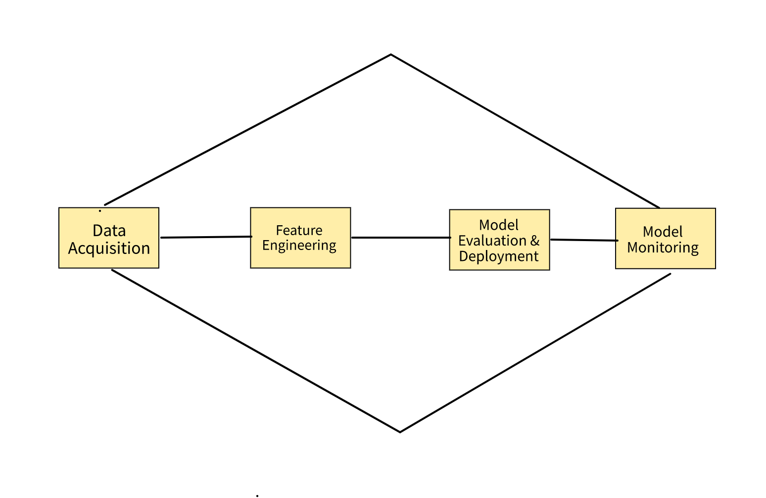
This post will demystify the MLOPs process. Models run in production, not Jupiter notebooks. Production is any environment where the models directly support a business function. The framework for operationalizing machine learning models successfully rests on four fundamental pillars. The pillars are data acquisition, curation, and labeling, Feature engineering and experimentation, model evaluation and deployment, and finally monitoring production for performance drops and drifts. The major unique challenge around MLOPs is its focus on developing, deploying, and sustaining models or artifacts derived from data which also need to reflect changes to data over time.
1. Data Acquisition, Curation, And Labelling
MLOPs pipelines start with data acquisition. The data could be sourced from public datasets, scraped, or collected from instrumenting applications or products with rich logs, data augmentation techniques like synonym replacement, word removal, multi-language translation, etc could be used to augment a sparse dataset. The most important thing is the availability of data with information relevant to the problem the model intends to solve.
The data acquired most times needs to be extracted from its's source for e.g PDFs contain tables, figures, and texts that have answers to questions so the next step in the pipeline after acquiring the PDF data is extracting the data from the source.
Post data extraction there is cleaning and preprocessing to remove noise the methods used are specific to the ML tasks for e.g in a Natural language processing application most of the preprocessing would be removing stop words (common words like is, a, or etc), stemming i.e removing a part of a word, or reducing a word to its stem or root. e.g cars -> car, lemmatization i.e converting the word to its base or root e.g walked, walking -> walk basically group different words by context, text normalization i.e representing the text and all its variations into one representation e.g 9 -> nine, etc.
There are other preprocessing steps unique to different branches of Machine learning, most of my experience is in the domain of natural language processing and my examples reflect this. Finally labeling the cleaned data is the last step in this phase. Labeling can be outsourced or performed by a team of in-house annotators. Most times the machine learning engineer and data science teams will have a subject matter expert working alongside them to make sure the labels are correct.
2. Feature Experimentation and Engineering
ML is experimental in nature, it's beneficial to prototype ideas quickly and only the best of the best ideas get into production. This phase deals with trying out ideas to improve the model's performance. Features are heavily inspired by the task at hand alongside domain knowledge. The experiments could be data or model-driven. The experiment is data-driven when we add, update or remove a feature or features.
The experiment is model driven when the model architecture changes for e.g changing from a tree-based model to a neural network etc. In deep learning pipelines the model learns features from the raw data fed into it, the drawback of this is the model becomes a black box as we lose interpretability of its results. Modeling usually starts from simple heuristics which become the features of the model. Sometimes stacking models in which one model output is the input to the other is another approach although as product feature grows model complexity grows also as part of a large product.
There is also transfer learning where preexisting knowledge from a big well-trained model is transferred to a newer model at its initial phase and then afterward the new model slowly adapts to the task at hand. The BERT model used in the NLP task of question answering is a good example of this.
Good feature engineering is a collaborative process, as most good ideas result from the collaboration of project stakeholders. Plausible ideas that could enable the model to make better predictions should be proactively sourced. The data science team and domain experts typically work together on this.
Iterate quickly over the acquired data, if the performance isn't up to the desired metric, evaluate other models. Some general tips in this phase are, to favor small changes over larger changes. Small code changes can hasten the code review process, it's easier to track the change in performance and revert the changes if performance is degraded post-change. The loop of faster code reviews, quicker feature validation, and fewer merge conflicts flow with the iterative nature of machine learning. It is important to use config files rather than editing the script file, the fewer changes made to the code base the better. These config files should be linked to the model training script. This method of constraining engineers to config changes can reduce bugs from new versions of code, libraries, data, etc.
3. Model Evaluation & Deployment
Before a model is deployed it is typically evaluated by a computing metric e.g (the number of correct predictions made by a model in relation to the total number of predictions made. We calculate it by dividing the number of correct predictions by the total number of predictions), mean squared error (measures the average squared difference between the estimated values and what is estimated, the lower the value the better with 0 = the model is perfect).
A typical evaluation metric could, for instance, be computed over a collection of labeled data points hidden at training time or a validation dataset to see if its performance is better than the currently running production model achieved during its own evaluation phase.
Model Evaluations are intrinsic and extrinsic. Intrinsic evaluation happens internally by the AI team while extrinsic evaluation occurs post-deployment externally by the end user etc. Intrinsic evaluation is a proxy for extrinsic evaluation, it's not a reliable proxy because we can't know the model performance till it's actually deployed and in use operationally.
Deploying the model is a multi-staged process and some of the stages in the deployment phase involve reviewing the proposed changes, staging the changes to increasing percentages of the users, or conducting A/B testing on users. A/B testing is simply split testing via a randomized process wherein multiple versions of an application in this instance the model is shown to different segments of application visitors at the same time to determine which version has the maximum impact and drives business metrics.
It is always good practice to keep a record of changes made in case there is a need to roll back. Data, product, business use case, user, and organization changes. Use dynamic datasets for validation. The validation datasets should reflect live data as much as possible, the model performance can be evaluated properly pre-deployment if the dataset used in the evaluation is close enough to live data. There are other practices prescribed like queuing every failed prediction for routine analysis later. Similarly, data should be collected to be used offline for offline validation in future iterations of the product lifecycle. Validation systems should be standardized for consistency, these defined validation standards would ensure the success of our evaluation system.
4. Monitoring Production For Performance Drops and Drifts
This phase is concerned with sustaining the models in production. As with everything in life, the model's post-deployment face some wear and tear issues like drift error and unpredictable bugs, etc. Drift error is bound to occur over time as the model gets new data different from the training set data. There are other unpredictable bugs sometimes there is a large discrepancy between offline validation accuracy and production accuracy immediately after deployment. Thus it's important the pipeline has high observability to catch failures immediately.
To know what bugs to focus on, we need to know when models are precisely underperforming to then map performance drops to the bugs but to know when models are underperforming means to identify bugs beforehand. This chicken-egg problem is a particular pain point of this phase but there are some strategies we can adopt to aid us in this phase.
Live metrics should be tracked using queries, and dashboards. Segment certain users to investigate prediction quality. The model should be patched with heuristics (rule) for known failure modes. Source other failure modes from the wild and add them to the evaluation set.
It is important to create new versions of models frequently retrained on labeled live data. ML bugs can be detected by tracking pipeline performance metrics like prediction accuracy and triggering an alert if there's a drop in performance exceeding a certain threshold. Model retraining cadence can range from hourly to every few months. The old version of the model should be maintained as a fallback model. This helps to reduce downtime when a production. Maintain layers of heuristics for e.g filter rules to stop noise to and from the model, simple fail-proof rules, etc. The data going in and out of pipelines should be validated. There are some simple metrics such as having hard constraints on features columns, placing hard bounds on values where they exist for example we can’t have negative values for age and weights, etc, and checking for completeness of the features via the fraction of nonnull values to null values, etc.
Conclusion
In summary, most of MLOP's pain points are down to factors such as a mismatch of the development and production environment. The development environment prioritizes high experimentation velocity so hypotheses can be verified and validated quickly. Jupyter notebook is good for the velocity of development but buggy and unscalable in production. To add more complexities, most software engineering practices are contradictory to the agility of analysis and exploration, code review may not have value in an ML-specific context but general software best practices should still be adhered to. The data errors found in the ML process range on a spectrum, there are hard errors for e.g swapping columns or violating constraints (negative age value for instance) these results in bad predictions. There are soft errors for e.g few null valued features in one data point these are hard to catch and quantify and the model still yields good enough predictions. It's expensive for users to see errors therefore changes should be quickly tested and bad ideas pruned early so monitoring the pipeline for bugs as early as possible so validation can happen earlier is also recommended. It is not possible to anticipate all bugs before they occur, it's helpful to store and manage multiple versions of production models and datasets for querying, debugging, and minimizing production pipeline downtime. ML engineers can respond to buggy production models by switching to a simpler, historical, or retrained version. ML is successful due to experimentation and iterating quickly on ideas. Effectively managing these three properties velocity, validation, and versioning will contribute to deployment success.